Network analysis
[1]:
import movekit as mkit
import numpy as np
import pandas as pd
import matplotlib.pyplot as plt
from scipy.spatial import Voronoi, voronoi_plot_2d, convex_hull_plot_2d, delaunay_plot_2d
import networkx as nx
import collections
[2]:
path = "datasets/fish-5-cleaned.csv"
data = mkit.read_data(path)
data = mkit.extract_features(data)
data.head()
Extracting all absolute features: 100%|██████████| 100.0/100 [00:01<00:00, 61.85it/s]
[2]:
| time | animal_id | x | y | distance | direction | turning | average_speed | average_acceleration | stopped | |
|---|---|---|---|---|---|---|---|---|---|---|
| 0 | 1 | 312 | 405.29 | 417.76 | 0.0 | (0.0, 0.0) | 0.0 | 0.210217 | -0.006079 | 1 |
| 1 | 1 | 511 | 369.99 | 428.78 | 0.0 | (0.0, 0.0) | 0.0 | 0.020944 | 0.000041 | 1 |
| 2 | 1 | 607 | 390.33 | 405.89 | 0.0 | (0.0, 0.0) | 0.0 | 0.070235 | 0.000344 | 1 |
| 3 | 1 | 811 | 445.15 | 411.94 | 0.0 | (0.0, 0.0) | 0.0 | 0.370500 | 0.007092 | 1 |
| 4 | 1 | 905 | 366.06 | 451.76 | 0.0 | (0.0, 0.0) | 0.0 | 0.118000 | -0.003975 | 1 |
Obtaining a list of graphs, based on delaunay triangulations
Caclulate a network list for each timestep based on delaunay. trinangulation. Each timestep carries the respective graph with data attached to nodes, edges and graph. Just insert time and animal specific x and y coordinate data.
[3]:
#Calculates a network list for each timestep based on delaunay triangulation (currently only one available)
graphs = mkit.network_time_graphlist(data)
Calculating spatial objects: 100%|██████████| 1000/1000 [00:12<00:00, 82.05it/s]
Computing euclidean distance: 100%|██████████| 1000/1000 [00:03<00:00, 263.66it/s]
Extracting all absolute features: 100%|██████████| 100.0/100 [00:01<00:00, 75.25it/s]
Calculating centroid distances: 100%|██████████| 1000/1000 [00:05<00:00, 182.21it/s]
Calculating centroid distances: 100%|██████████| 1000/1000 [00:06<00:00, 162.88it/s]
Calculating centroid distances: 100%|██████████| 1000/1000 [00:04<00:00, 210.44it/s]
Computing centroid direction: 100%|██████████| 100.0/100 [00:00<00:00, 709.71it/s]
Calculating network list: 100%|██████████| 1000/1000 [00:04<00:00, 226.92it/s]
[4]:
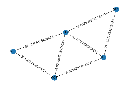
# Visualizing the graph for time step '3'-

pos = nx.spring_layout(graphs[2])

nx.draw(graphs[2], pos)
node_labels = nx.get_node_attributes(graphs[2], 'animal_id')
nx.draw_networkx_labels(graphs[2], pos=pos, labels=node_labels)

edge_labels = nx.get_edge_attributes(graphs[2], 'distance')
nx.draw_networkx_edge_labels(graphs[2], pos=pos, edge_labels=edge_labels)
plt.show()
[5]:
# Display all graph attributes at time 3
graphs[2].graph
[5]:
{'time': 3,
 'x_centroid': 395.392,
 'y_centroid': 423.234,
 'medoid': 312,
 'polarization': 0.30008793109871296,
 'total_dist': 1.0251553045775692,
 'mean_speed': 0.15561007599508753,
 'mean_acceleration': 0.0018184129934008715,
 'mean_distance_centroid': 29.691399999999998,
 'centroid_direction': (0.01, 0.014)}
[6]:
# Display all edges at time 3
graphs[2].edges
[6]:
EdgeView([(312, 811), (312, 607), (312, 511), (312, 905), (811, 905), (811, 607), (607, 511)])
[7]:
# Display the distance of one node pair at time 3
graphs[2].edges[312, 811]
[7]:
{'distance': 40.70507585056191}
[8]:
# Display all attributes of node 312 at time 3
graphs[2].nodes[312]
[8]:
{'time': 3,
 'animal_id': 312,
 'x': 405.31,
 'y': 417.07,
 'distance': 0.30000000000001137,
 'direction': (0.0, -0.3),
 'turning': 0.9986876634765885,
 'average_speed': 0.17472339975245438,
 'average_acceleration': -0.004658902224371936,
 'stopped': 1,
 'x_centroid': 395.392,
 'y_centroid': 423.234,
 'medoid': 312,
 'distance_to_centroid': 11.677}
Network analysis
The networkx package enables to analyze the extracted graphs over time. See doc: https://networkx.org/documentation/stable/index.html
[9]:
len(graphs)
[9]:
1000
[10]:
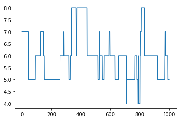
# Plot number of nodes over time
num_edges = []
for G in graphs:
    num_edges.append(nx.number_of_edges(G))

plt.plot(num_edges)
plt.show()
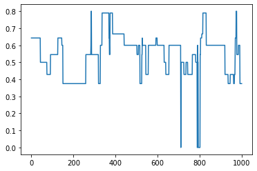
[11]:
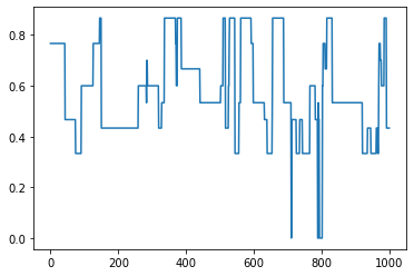
# Plot clustering coefficient over time
avg_cluster = []
for G in graphs:
    avg_cluster.append(nx.average_clustering(G))

plt.plot(avg_cluster)
plt.show()
[12]:
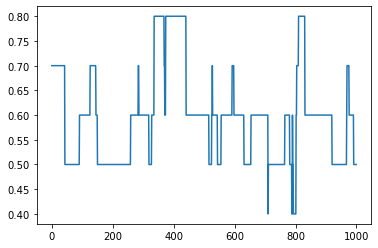
# Plot density over time
dens = []
for G in graphs:
    dens.append(nx.density(G))

plt.plot(dens)
plt.show()
[13]:
# Plot transitivity over time
trans = []
for G in graphs:
    trans.append(nx.transitivity(G))

plt.plot(trans)
plt.show()
Compute features for individiual nodes
[14]:
# Pick the first graph
G = graphs[0]
[15]:
# Degree
dict(G.degree())
[15]:
{312: 4, 811: 3, 905: 2, 607: 3, 511: 2}
[16]:
# Degree centraility
nx.degree_centrality(G)
[16]:
{312: 1.0, 811: 0.75, 905: 0.5, 607: 0.75, 511: 0.5}
[17]:
# Clustering coefficient
nx.clustering(G)
[17]:
{312: 0.5,
 811: 0.6666666666666666,
 905: 1.0,
 607: 0.6666666666666666,
 511: 1.0}
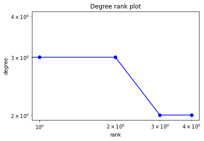
[18]:
# Degree rank
degree_sequence = sorted([d for n, d in G.degree()], reverse=True)
dmax = max(degree_sequence)

plt.loglog(degree_sequence, "b-", marker="o")
plt.title("Degree rank plot")
plt.ylabel("degree")
plt.xlabel("rank")
plt.show()
For more methods please check the networkX doc: https://networkx.org/documentation/stable/index.html
[ ]: